Audio Separation Using Principal Component Analysis (PCA)

In this project, I perform audio separation through of mixed signal through implementation of Variational Mode Decomposition and Principal Component Analysis (PCA). It is seen that mixture of pure sinusoids of different frequencies is separated very efficiently while that of instruments – cymbals and bass drums are separated only satisfactorily. Comparison of original and unmixed (separated) signal is made through various metrics such as correlation coefficient, percentage error, root mean square error and visually by spectrographs. A brief overview of audio acquisition, representation and storage is also provided.

Audio Acquisition, Representation and Storage

Audio acquisition is the process of converting the physical phenomenon we call sound into a format suitable for digital processing, representation involves extracting from the sound, information necessary to perform a specific task, and the storage is the task of encoding the acoustic signals suitably [1]. A typical sound wave can be represented by:

$s(t) = sin(\mathrm{2\pi f t}+\phi) = sin(\frac{2\pi t}{T} + \phi)$

where $A$ is called the amplitude and it represents the maximum distance from equilibrium position, $\phi$ is the phase, $T$ is called period which is the time interval length between two instances of $s(t)$ . Also, $f = 1/T$ is the frequency measured in Hz. The only sounds that are used in audio applications are those that can be perceived by human beings. The intensities can be measured through the ratio $I/I_0$ , where $I_0$ is the threshold of hearing (THO) viz. the minimum intensity that can be detected by human ears. However, this is problematic as the value of $I/I_0$ corresponds to $10^{-12} W/m^2$ , while the maximum value of $I$ that can be tolerated without permanent physiological damages is $I_{max} = 10^3 W/m^2$ . The ratio $I/I_0$ can thus range across 15 orders of magnitude and this makes it difficult to manage different intensity values. Hence, the ratio $I/I_0$ is measured using the deciBel (dB) scale, where the intensity measure in dB $I^*$ is given as.

$I^* = 10\log_{10}(\frac{I}{I_0})$

Audio Acquisition – Sampling

In the process of sampling, the displacement of measurement membrane is measured at regular time steps. The number $F$ of measurements per seconds is called sampling frequency or sampling rate and the time interval $T_c = 1/F$ between two consecutive measurements is called sampling period. The relationship between the analog signal $s(t)$ and the sampled signal $s[n]$ is as follows:

$s[n] = s(nT_c)$

where the square brackets are used for sampled discrete-time signals and the parentheses are used for continuous signal. A common rule of thumb when deciding upon the sampling frequency can be ascertained by the Nyquist or Shannon frequency, given as $> 2f_(max)$ , here $f_(max)$ is the highest frequency represented in the sound signal. The following table shows common sampling rates along with bandwidth:

Sound Quality/Type	Sampling Rate (Hz)	Bandwidth
Telephone	8000	200 Hz – 3.4 kHz
CD Audio	44100	5 Hz – 20 kHz
DAT Audio	48000	5 Hz – 20 kHz
DVD Audio	96000	0 Hz – 96 kHz
DVD Audio with sterio-mixes	196000	0 Hz – 96 kHz

Table: Common sampling rates and bandwidths

Audio Representation

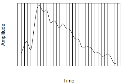
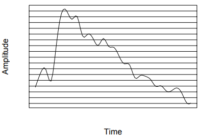
Since sound is longitudinal pressure wave it consists of continuous values as opposed to discreet ones. Since most signal processing is handled by digital devices it is necessary to digitize sound. Digitization implies conversion to a stream of numbers, preferably integers for increased processing efficiency [2]. Sampling in the amplitude or voltage dimension is called quantization. The most straightforward method to perform such a task is known as pulse code modulation (PCM). It involves three steps viz. sampling, quantization (Linear or non-linear) and coding (A-Law or -Law). The figures below can be used to conceptualize sampling and quantization:

Figure: Sampling the analog signal in time

Figure: Quantization is ‘sampling’ the analog signal in amplitude [2]

Audio Storage

The number of bits used to represent audio samples has an important role in storage and transmission. The higher the number of bits, the larger is the memory space needed to store a recording and transmit through a channel. The number of bits per unit time necessary to represent a signal is called bit-rate. The area dealing with reducing bit-rate while at the same time preserving quality of the signal is called audio encoding. The primary encoding methods result in audio formats such as MPEG, WAV, mp3, etc. The below table provides more information on different encoding formats.

Audio Format	Sampling Rate (kHz)	Bit Rate (kbits/s)
MPEG – 1	32 – 48	32 – 384
MPEG – 2	16 – 24	8 – 144
WAV	8 – 48	4.8 – 176
MP3	8 – 44	8 – 320

Table: Common audio formats with sampling and bit rate

Blind Source Separation

Blind source separation (BSS) is the extraction of single constituent sound sources that comprise a mixture of signals and as such has several applications in bio-medical signal processing, speech processing, speech recognition, communications, etc. To create such a mixture the independent source signals are usually multiplied with different weights (mixing matrix) and the summed mixture is recorded. The source signals are expected to be recovered only from the available mixture of the signal with no other background knowledge. This is often compared to the ‘Cocktail Party Effect’ which is the ability of human brain to focus on specific human voice, while filtering out other voices or backgrounds [3,4]. In this particular article we will concentrate on single channel blind source separation (SCBSS).

A Brief Overview of Blind Source Separation Paradigms

Several methods have been proposed for single channel blind source separation (SCBSS) in literature. In [5], single channel-independent component analysis (SCICA) has been used to separate the sources. A new method based on wavelet transform along with FastICA has been used in [6]. In [7], the technique of ensemble empirical mode decomposition (EEMD) has been used to decompose a single observation into a number of intrinsic mode functions (IMFs). Principle component analysis (PCA) was used to select the required number of IMFs to select the required number of IMFs to be given as input to ICA algorithm. A learning framework has been applied to blind source separation (BSS) in [8], which treats BSS as a generalized eigenvalue problem. Our project deals with SCBSS employing variational mode decomposition (VMD) and PCA.

Variational Mode Decomposition (VMD)

VMD decomposes a signal into a number of modes concurrently and non-recursively such that the combination of all the modes can reconstruct the original signal. It also searches for the center frequency of the modes and each mode is band-limited about this center frequency. Thus, it decomposes a real valued signal into a finite number of modes simultaneously. These modes have specific sparsity properties and the center frequency is also determined along with the modes. Each of the modes are compact around its center frequency. The bandwidth of each mode and reconstruction fidelity are controlled by different parameters. Details of VMD implementation can be found later in the text.

Principal Component Analysis (PCA)

This procedure is called the Principal Component Analysis (PCA), Proper Orthogonal Decomposition (POD) or the Karhunen-Loeve Decomposition. PCA identifies the dynamics and behavior of a system from a seemingly complex and incoherent set of data. Even without any prior knowledge of governing systems we can produce low level reductions. PCA can be done by eigenvalue decomposition of a data covariance matrix or singular value decomposition (SVD) of a data matrix, usually after mean centering and normalizing the data matrix for each attribute.

Figure: PCA of a multivariate Gaussian distribution

If we imagine a random set of n-dimensional data, then PCA can be visualized as transforming that data into a n-dimensional ellipsoid with its axes serving as each of the principal components. When the axis of the ellipsoid is small, then the variance along that axis is also small, and by omitting that axis and its corresponding principal component from our representation of the data-set, we lose only a small amount of information. Thus, we can achieve reduction and identification/characterization of data from PCA.

Proposed Method

In this work, a mixture of two sources $x_1(t)$ and $x_2(t)$ has been considered. The single channel containing the mixture of these two sources is given by:

$x(t)=a_1x_1(t)+a_2x_2(t)+n(t)$

Here, $a_1$ and $a_2$ are weighting coefficients and $n(t)$ is any noise that may be introduced in the system. Our objective is to extract $x_1(t)$ and $x_2(t)$ . The proposed method consists of applying VMD on $x(t)$ and thus decomposing it into $n$ number of modes. Each mode belongs to a different spectral band. If the signal $x(t)$ is a mixture of source signals belonging to different spectral bands, then they are captured by the different modes in VMD. Not only that, the out-band high frequency noise gets captured in other modes. If the noisy modes are rejected, then the remaining modes are the extracted source signals. For selecting the required signals modes PCA is used. PCA transforms a set of observed correlated vectors to set of uncorrelated vectors. The transformation is as follows:

$y = A^Tx$

where, $A$ is known as orthogonal matrix, $x$ is the set of correlated vectors and $y$ is the set of uncorrelated vectors. The elements of the vector set are called the principal components. These principal components of $y$ are maximized under the constraint that their principal component vectors are orthogonal to each other. Only the first $m$ principal components (where $m$ is the number of source signals), corresponding to the highest eigenvalues are selected. The eigenvalues corresponding to the modes containing noise would be much less as compared to the ones containing the source signals. Thus, PCA helps to select the m modes which directly gives the source components.

Algorithm for the proposed method

1. Input observed signal $x(t)$

2. Apply VMD on x(t) to get n modes: $M_1, M_2$ up to $M_n$

3. Apply PCA on $M_1$ to $M_n$ to select $m$ principal components: $P_1, P_2$ up to $P_m$

4. Extracted sources: $P_1, P_2$ up to $P_m$

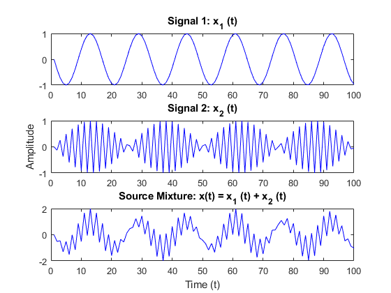
Signal (Constructed) – Pure Sinusoids

We first use pure sinusoids of different frequencies to test the accuracy of the proposed method. In this implementation $x_1(t) = sin(3t)$ and $x_2(t) = sin(7t)$ . The below figure shows the individual signals and their mixture.

Figure: Pure sinusoids and their mixture

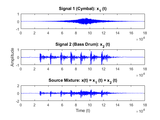
Signal (Constructed) – Instruments Cymbal and Bass Drum

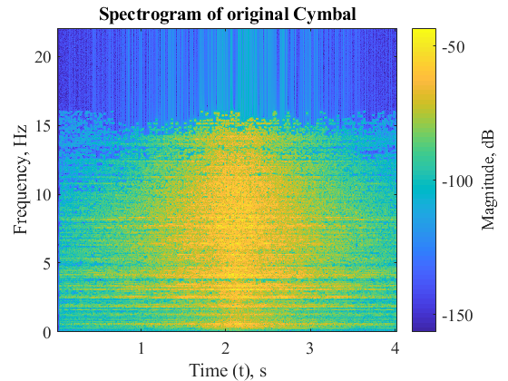
Signals for Cymbals and Bass are shown below. These instruments are chosen as they operate in non-overlapping frequency range. Cymbals operate in the range 3 to 5 kHz and bass drums between 60 to 100 Hz.

Figure: Sound signal for cymbal, bass drum and their mixture

Algorithm Implementation

As described earlier, variational mode decomposition is applied on the single channel mixed signal $x(t)$ to decompose it into $K$ band separated modes. For each type of signal $K$ is kept 2 as it is believed to a combination of two dominant modes. The function $\mathrm{VMD()}$ contributed by authors in [9,10] is used for this purpose. Principal components of the $K$ modes modes is found out by implementing inbuilt Matlab function $\mathrm{pca()}$ . The signal reconstruction can be obtained by using the following equation:

$\mathrm{PCA}\: \mathrm{reconstruction} = \mathrm{PC}\: \mathrm{scores}\times \mathrm{Eigenvectors^T}+ \mathrm{Mean}$

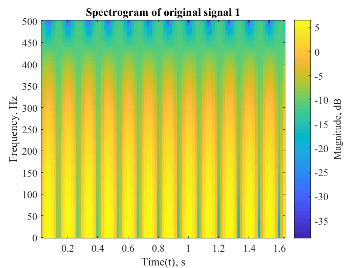
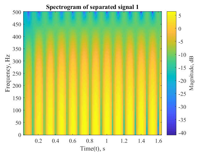
Result – Separation of Pure Sinusoids

Results obtained from the implementation of the above algorithm for separation of pure sinusoidal mixed signals are shown below. Data is shown in both in terms of amplitude and frequency (spectrogram) versus time for effective comparison.

Figures: Separated and original signal 1 of mixture of pure sinusoids

Figure: Spectrogram of original signal 1 of mixture of pure sinusoids

Figure: Spectrogram of separated signal 1 of mixture of pure sinusoids

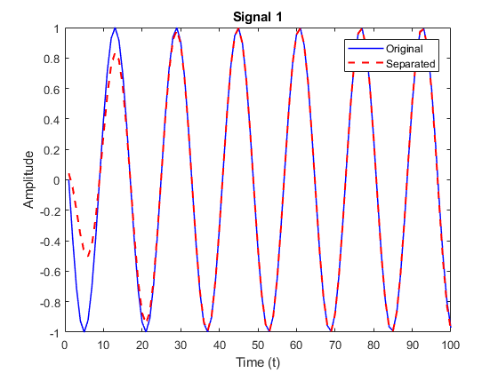
The following metrics were calculated to determine the efficiency of the separation algorithm for signal 1 of mixture of pure sinusoids:

Correlation coefficient	0.9872
Percentage error	6.3593
Root mean square error	0.0187

Figures: Separated and original signal 2 of mixture of pure sinusoids

Figure: Spectrogram of original signal 2 of mixture of pure sinusoids

Figure: Spectrogram of separated signal 2 of mixture of pure sinusoids

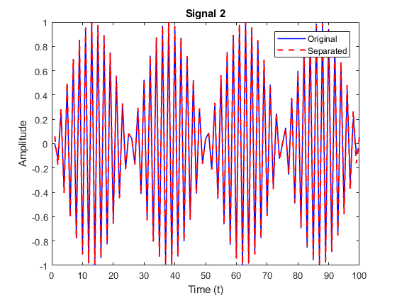
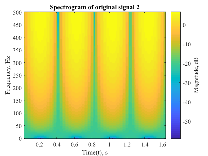
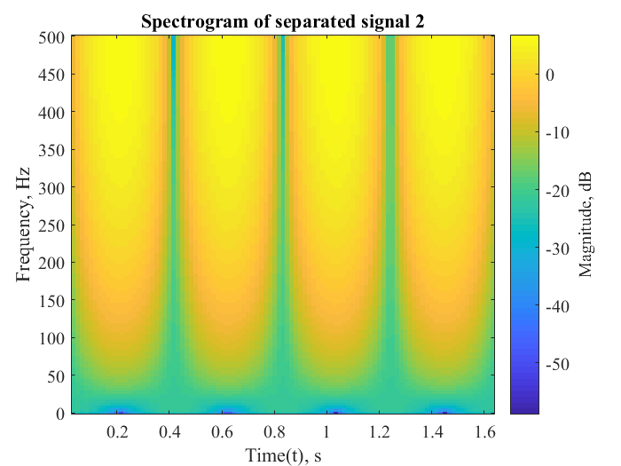
The following metrics were calculated to determine the efficiency of the separation algorithm for signal 2 of mixture of pure sinusoids:

Correlation coefficient	0.9987
Percentage error	4.5866
Root mean square error	0.0053

Result – Separation of Cymbal and Bass Drum

The following results are obtained for separation of cymbal and bass drum constituent signals from the mixture.

Figures: Separated and original signal 1 of mixture of Cymbal and Bass Drum

Figure: Spectrogram of original signal 1 of mixture of Cymbal and Bass Drum

Figure: Spectrogram of separated signal 1 of mixture of Cymbal and Bass Drum

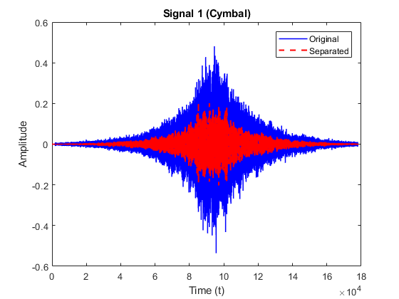
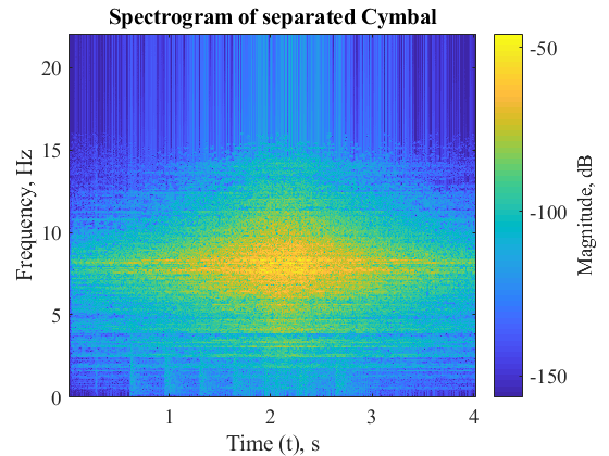
The following metrics were calculated to determine the efficiency of the separation algorithm for signal 1 (Cymbal) of mixture of Cymbal and Bass Drum:

Correlation coefficient	0.6794
Percentage error	43.9026
Root mean square error	0.1601

Figures: Separated and original signal 2 of mixture of Cymbal and Bass Drum

Figure: Spectrogram of original signal 2 of mixture of Cymbal and Bass Drum

Figure: Spectrogram of separated signal 2 of mixture of Cymbal and Bass Drum

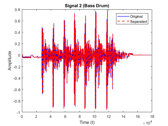
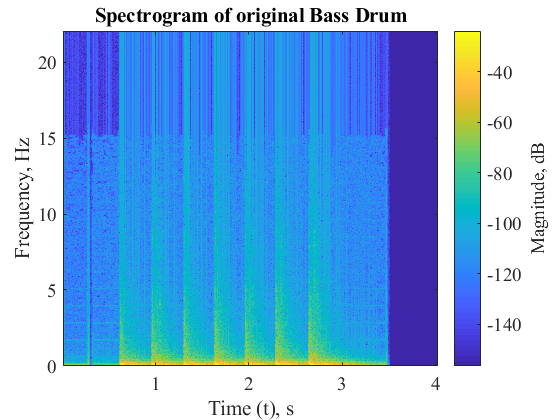
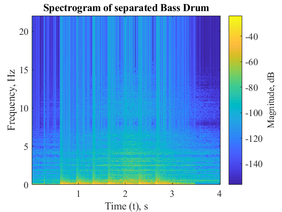
The following metrics were calculated to determine the efficiency of the separation algorithm for signal 2 (Bass Drum) of mixture of Cymbal and Bass Drum:

Correlation coefficient	0.9988
Percentage error	16.4570
Root mean square error	0.0489

Discussion

As we can see for the results section, pure sinusoids are separated very efficiently by the mentioned algorithm. This behavior is anticipated as they are created through addition of pure sinusoids comprising of one dominant frequency each. However, the separation of Cymbals and Bass Drum is not very efficient. This can be attributed to the presence of several frequency modes and noise that might be introduced during recording of Cymbals and Bass Drum. The algorithm thus fairly performs separation and has scope for further improvement.

Matlab Code

% ME 535 Project
% Analysis of Audio using PCA
clear all;close all, clc
t = linspace(0, 6000, 100);
fs = 1; %44100
s1 = sin(3*t)'; %Trying to seperate this and s2
%[s,fs] = audioread('cymbal_recording_clip.mp3');
%s_2 = s(:,1);
s2 = sin(7*t)'; %s_2(3000:3999)';
mix = s1'+ s2'%0.3*s1'+ 0.7*s2';

figure(1)
subplot(3,1,1)
plot(s1,'-b'); title('Signal 1: x_1 (t)')
subplot(3,1,2)
plot(s2,'-b'); title('Signal 2: x_2 (t)')
ylabel('Amplitude');
subplot(3,1,3)
plot(mix,'-b'); title('Source Mixture: x(t) = 0.3x_1 (t) + 0.7*x_2 (t)');
xlabel('Time (t)');

%%
% Implementation of VMD
alpha = 2000;       % moderate bandwidth constraint
tau = 0;            % noise-tolerance (no strict fidelity enforcement)
K = 2;              % K modes
DC = 0;             % no DC part imposed
init = 1;           % initialize omegas uniformly
tol = 1e-7;

[u, u_hat, omega] = VMD(mix, alpha, tau, K, DC, init, tol)
% u       - the collection of decomposed modes
% u_hat   - spectra of the modes
% omega   - estimated mode center-frequencies

figure(2)
plot(u); title('u')

figure(3)
plot(u_hat);title('u-hat')

figure(4)
plot(omega); title('omega')

%%
% Implementation of PCA and Signal Reconstruction
close all;

[coeff, score, latent, tsquared, explained, mu] = pca(u);
%coeff = pca(u')
recon = score*coeff'+repmat(mu,K,1)

figure(5)
plot(s1,'-b', 'Linewidth',1.1)
hold on;xlabel('')
plot (recon(1,:),'--r', 'Linewidth',1.5);
xlabel('Time (t)');ylabel('Amplitude');
title('Signal 1')
legend('Original', 'Separated')

figure(6)
plot(s2,'-b', 'Linewidth',1.1)
hold on;
plot (recon(2,:),'--r', 'Linewidth',1.5);
xlabel('Time (t)');ylabel('Amplitude');
title('Signal 2')
legend('Original', 'Separated')

%%
% Spectrogram of Original Signal (s1)

figure(7)
spectrogram(s1, 4, 3/4*4, [], fs, 'yaxis')
box on
set(gca, 'FontName', 'Times New Roman', 'FontSize', 14)
xlabel('Time, s')
ylabel('Frequency, Hz')
title('Spectrogram of sin(3t)-original')

h = colorbar;
set(h, 'FontName', 'Times New Roman', 'FontSize', 14)
ylabel(h, 'Magnitude, dB')

%%
% Spectrogram of Reconstructed Signal (s1)

figure(8)
spectrogram(recon(1,:), 1024, 3/4*1024, [], fs, 'yaxis')
box on
set(gca, 'FontName', 'Times New Roman', 'FontSize', 14)
xlabel('Time, s')
ylabel('Frequency, Hz')
title('Spectrogram of sin(3t)-unmixed')

h = colorbar;
set(h, 'FontName', 'Times New Roman', 'FontSize', 14)
ylabel(h, 'Magnitude, dB')

%%
% Spectrogram of Original Signal (s2)

figure(9)
spectrogram(s2, 1024, 3/4*1024, [], fs, 'yaxis') %1024 or 4
box on
set(gca, 'FontName', 'Times New Roman', 'FontSize', 14)
xlabel('Time, s')
ylabel('Frequency, Hz')
title('Spectrogram of sin(7t)-original')

h = colorbar;
set(h, 'FontName', 'Times New Roman', 'FontSize', 14)
ylabel(h, 'Magnitude, dB')

%%
% Spectrogram of Unmixed Signal (s2)

figure(10)
spectrogram(recon(2,:), 1024, 3/4*1024, [], fs, 'yaxis')
box on
set(gca, 'FontName', 'Times New Roman', 'FontSize', 14)
xlabel('Time, s')
ylabel('Frequency, Hz')
title('Spectrogram of sin(7t)-unmixed')

h = colorbar;
set(h, 'FontName', 'Times New Roman', 'FontSize', 14)
ylabel(h, 'Magnitude, dB')

%%
% Metrics for comparison
R_1 = corrcoef(s1,recon(1,:))
R_2 = corrcoef(s2,recon(2,:))
Norm_s1 = norm(s1-recon(1,:));

per_err = 100*((spectrogram(s1)-spectrogram(recon(1,:))))./spectrogram(s1);
per_err_abs = abs(per_err);
per_err_vector = per_err_abs(:)

%RMS error signal
RMSE = sqrt(mean((s1 - recon(1,:)).^2))

%RMS error spectrogram
RMSE = mean(abs(sqrt(mean((spectrogram(s1) - spectrogram(recon(1,:))).^2))))
%mean_percentage_error = mean(per_err_vector)

References

[1] Camastra, Francesco and Vinciarelli, Alessandro. “Machine Learning for Audio, Image and Video Analysis.” Advanced Information and Knowledge Processing, Springer-Verlag, London (2015).

[2] Li, Ze-Nian., Drew, Mark S. and Liu, Jiangchuan. Fundamentals of Multimedia. Springer International Publishing, Switzerland (2003).

[3] Dey, Priyanka., Satija, Udit and Ramakumar, Barathram. “Single Channel Blind Source Separation Based on Variational Mode Decomposition and PCA.” Proceedings of the Annual IEEE India Conference (INDICON). New Delhi, India, December 12-20, 2015.

[4] Deep Learning Machine Solves the Cocktail Party Problem, Online: https://www.technologyreview.co-m/s/537101/deep-learning-machine-solves-the-cocktail-party-problem/, Accessed: 5/25/2018 3:28 PM.

[5] Davies, Mike and James, Christopher. “Source separation using single channel ICA.” Signal Processing. Vol. 87 No. 8 (2007): pp. 1819-1832. DOI
10.1016/j.sigpro.2007.01.011.

[6] Lopez, Ma., Lozano, Meron M., Sanchez, Luis P. and Moreno, Noe O. “Blind Source Separation of audio signals using independent component analysis and wavelets” Proceedings of the International Conference on Electrical Communications and Computers. San Andres Cholula, Mexico, February 28 – March 2, 2011.

[7] Guo, Yina., Huang, Shuhua and Li, Yongtang. “Single-Mixture source separation using dimensionality reduction of ensemble empirical mode decomposition and independent component analysis.” Circuits, Systems, and Signal Processing. Vol. 31 No. 6 (2012): pp. 2047-2060.

[8] Liu, Hailin and Cheung, Yiuming. A Learning Framework for Blind Source Separation Using Generalized Eigenvalues. In: Wang J., Liao XF., Yi Z. (eds) Advances in Neural Networks. Lecture Notes in Computer Science. Vol. 3497. Springer, Berlin, Heidelberg. DOI https://doi.org/10.1007/11427445_77.

[9] Dragomiretskiy, Konstantin and Zosso, Dominique. “Variational Mode Decomposition. Online: https://www.mathworks.com/matlabcent-ral/fileexchange/44765-variational-mode-decomposition, Accessed: 5/26/2018 5:18 PM.

[10] Dragomiretskiy, Konstantin and Zosso, Dominique. “Variational Mode Decomposition.” IEEE Transactions on Signal Processing, Vol. 62 No. 2 (2013): pp. 531-544. DOI: 10.1109/TSP.2013.2288675.

Sameer Meshram

Welcome to my portfolio-cum-blog